Solution Techniques

Cluster-First Route-Second Method

These methods perform a single clustering of the vertex set and then determine a vehicle route on each cluster. We will describe the following algorithms:

Fisher and Jaikumar (1981)
The Petal algorithm
The Sweep algorithm
Taillard (1993)

Fisher and Jaikumar Algorithm

The Fisher and Jaikumar algorithm [Fisher and Jaikumar 1981] is well known. It solves a Generalized Assignment Problem (GAP) to form the clusters. The number of vehicles K is fixed. The algorithm can be described as follows:

Step 1. Seed Selection

Choose seed points $j(k)$ in V to initialize each cluster k.

Step 2. Allocation of Customers to Seeds

Compute the cost $c(ik)$ of allocating each customer i to each cluster k as $allocation cost formula$ .

Step 3. Generalized Assignment

Solve a GAP with costs $c(ik)$ , customer weights $d(i)$ and vehicle capacity Q.

Step 4. TSP Solution

Solve a TSP for each cluster corresponding to the GAP solution.

Petal Algorithm

A natural extension of the sweep algorithm is to generate several routes, called petals [Ryan, Hjorring and Glover 1993], and make a final selection by solving a set partitioning problem of the form:

$min sum of costs$

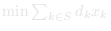
subject to:

$set partitioning constraints$

$x(k) = 0$ or 1 $k in S$ ,

where S is the set of routes, $x(k) = 1$ if and only if route k belongs to the solution, $a(ik)$ is the binary parameter equal to 1 only if vertex i belongs to route k, and $c(k)$ is the cost of petal k. If routes correspond to contiguous sectors of vertices, then this problem possesses the column circular property and can be solved in polynomial time (Ryan, Hjorring and Glover).

The Sweep Algorithm

The sweep [see] algorithm applies to planar instances of the VRP. It consists of two parts:

Split: Feasible clusters are initially formed by rotating a ray centered at the depot.
TSP: A vehicle route is then obtained for each cluster by solving a TSP.

Some implementations include a post-optimization phase in which vertices are exchanged between adjacent clusters, and routes are reoptimized. A simple implementation of this method is as follows, where we assume that each vertex i is represented by its polar coordinates $(θ, ρ)$ , where $θ$ is the angle and $ρ$ is the ray length. Assign a value $θ(i*) = 0$ to an arbitrary vertex $i*$ and compute the remaining angles from $angle formula$ . Rank the vertices in increasing order of their angles.

Step 1. Route Initialization

Choose an unused vehicle k.

Step 2. Route Construction

Starting from the unrouted vertex having the smallest angle, assign vertices to the vehicle k as long as its capacity or the maximal route length is not exceeded.

If unrouted vertices remain, go to Step 1.

Step 3. Route Optimization

Optimize each vehicle route separately by solving the corresponding TSP (exactly or approximately).

Taillard's Algorithm

Taillard's [Taillard 1993] algorithm defines neighborhoods using the $λ$ -interchange generation mechanism [Osman 1993]. Individual routes are reoptimized using the optimization algorithm of [Volgenant and Jonker 1993]. A novel feature of Taillard's algorithm is the decomposition of the main problem into subproblems.

In planar problems, these subproblems are obtained by initially partitioning vertices into sectors centered at the depot, and into concentric regions within each sector. Each subproblem can be solved independently, but periodic moves of vertices to adjacent sectors are necessary. This makes sense when the depot is centered and vertices are uniformly distributed in the plane.

For non-planar problems, and for planar problems not possessing these properties, the author suggests a different partitioning method based on the computation of shortest spanning arborescences rooted at the depot. This decomposition method is particularly well suited for parallel implementation, as subproblems can then be distributed among the various processors.

The combination of these strategies yields excellent computational results.