Problem Formulation

VRP Technical Description

The Vehicle Routing Problem (VRP) is a combinatorial optimization problem whose ground set is the edges of a graph G(V, E). The notation used for this problem is as follows:

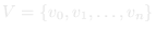is a vertex set, where:
- a depot is located at $v0$ ;
- $V′ = V \ {v0}$ is the set of $n$ customers (cities).
$A = {(vi, vj) :$ , i $≠$ j, is an arc set.
$C$ is a matrix of non-negative costs or distances $c_ij$ between customers $vi$ and $vj$ .
$d$ is a vector of the customer demands.
$R_i$ is the route assigned to vehicle $i$ .
$m$ is the number of vehicles (all identical). One route is assigned to each vehicle.

When $c_ij = c_ji$ for all $(vi, vj) ∈ A$ , the problem is said to be symmetric, and it is then common to replace $A$ with the edge set $E = {(vi, vj) | vi, vj ∈ V; i < j}$ .

With each vertex $vi$ in $V′$ is associated a quantity $q_i$ of goods to be delivered by a vehicle. The VRP thus consists of determining a set of $m$ vehicle routes of minimal total cost, starting and ending at the depot, such that every vertex in $V′$ is visited exactly once by exactly one vehicle.

For easy computation, one can define $lower bound on the number of vehicles$ , an obvious lower bound on the number of trucks needed to serve the customers in set V′.

We consider a service time $δ_i$ (the time needed to unload all goods) required by a vehicle to unload the quantity $q_i$ at $vi$ . The total duration of any vehicle route (travel plus service times) may not surpass a given bound $D$ , so in this context the cost $c_ij$ is taken to be the travel time between the cities. The VRP defined above is NP-hard [Lenstra & Rinnooy Kan 1981].

Feasible solutions and cost

A feasible solution is composed of:

a partition ${R1, …, Rm}$ of V;
a permutation $σ_i$ of $R_i ∪ {0}$ specifying the order of the customers on route $i$ .

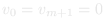The cost of a given route ( $R_i = (x0, x1, …, x_{m+1})$ ), where $x_i ∈ R_i$ and $x0 = x_{m+1} = 0$ (0 denotes the depot), is given by:

$F(R_i) = sum of c_{i,i+1} plus sum of δ_i$

A route $R_i$ is feasible if the vehicle stops exactly once at each customer and the total duration of the route does not exceed the prespecified bound $D$ :

$F(R_i) ≤ D$

Finally, the cost of the problem solution S is:

$F_VRP = sum over i=1..m of F(R_i)$

Integer programming formulation

Let x_ij be a binary variable equal to 1 if the arc from i to j is used by a vehicle, and 0 otherwise. The capacitated VRP can be written as the following two-index vehicle flow model:

min ∑_i∈V ∑_j∈V c_ij x_ij

subject to:

∑_i∈V x_ij = 1 ∀j ∈ V′ (each customer is entered exactly once)

∑_j∈V x_ij = 1 ∀i ∈ V′ (each customer is left exactly once)

∑_j∈V′ x_0j = ∑_i∈V′ x_i0 = m (m vehicles leave and return to the depot)

∑_i∈S ∑_j∈S x_ij ≤ |S| − r(S) ∀S ⊆ V′ (capacity-cut / subtour elimination)

x_ij ∈ {0, 1}

Here r(S) is a lower bound on the number of vehicles needed to serve the customer set S; in the capacitated case the simple bound ⌈∑_i∈S q_i / Q⌉ is typically used, where Q is the vehicle capacity.

A modern perspective (2026). State-of-the-art exact methods for the VRP — notably branch-cut-and-price algorithms that combine column generation with cutting planes — can now solve instances with a few hundred customers to proven optimality. For larger instances, heuristic and metaheuristic methods (such as those covered in our algorithms section) and hybrid matheuristics routinely produce high-quality solutions for problems with thousands of customers.